Historical Background
NMR is by far the most powerful form of spectroscopy to the practicing chemist, for two basic reasons. First of all, the hardware is extremely mature – the development of radiofrequency components for radar half a century ago, and extensive engineering since that time, has made it possible to create staggeringly complex excitation sequences. To select one particular problem, as a graduate student decades years ago I designed sequences of literally thousands of pulses, which forced molecules to absorb photons in groups. Modern NMR spectrometers (and their clinical counterparts, used for magnetic resonance imaging (MRI)) routinely give arbitrarily shaped (phase and amplitude modulated) radiofrequency pulses, and also routinely use magnetic field gradient pulses to suppress magnetization or obtain spatial resolution.
Of much greater importance, however, is the fact that the theoretical framework behind NMR and MRI is mature. Even twenty years ago, it was possible to calculate the effects of thousand-pulse sequences; when theory and experiment disagreed, it meant the spectrometer had to be fixed! No other modern spectroscopy has such a strong theoretical basis, which of course is used to understand the structures of molecules as complicated as proteins in solution, and which was recognized (for example) by Richard Ernst’s Nobel Prize in 1991.
We were thus startled to discover a major omission in this framework. Extremely simple pulse sequences, which could easily be shown theoretically to give no signal, experimentally give strong peaks even in very simple samples. In addition, the resonances are at different places than would be seen in the normal NMR spectrum. Consider, for example, the two pulse sequences in Figure 1. They both contain two radiofrequency pulses (in red) that rotate magnetization by 90 degrees, and they both contain magnetic field gradient pulses. The spectrum is obtained by acquiring the signal as a function of t1 and t2, then performing a two-dimensional Fourier transformation. The gradient in the interval t1 destroys the macroscopic magnetization, because molecules in different positions have different resonance frequencies. If there were a gradient pulse at the beginning of t2 with exactly the same area some magnetization might recover (this is a so-called “spin echo”) but instead another gradient pulse is given with twice the area, or no gradient pulse at all is given. In either case, all experimental signals should be suppressed. For this reason, these sequences are called CRAZED experiments; to an NMR spectroscopist, they look crazed.
Instead, peaks appear with about 10% of the macroscopic magnetization, giving a typical signal size 1000 times larger than the noise. Figure 1 shows spectra from a mixture of three molecules, each of which gives a single-line NMR spectrum. The three expected frequencies are seen in the directly detected dimension, but in the other dimension, peaks only occur at frequencies corre¬spon¬ding to flipping two spins on different molecules. This is disturbing to protein NMR spectroscopists, who use peaks with different frequencies in f1 and f2 (“crosspeaks”) to determine structural relationships within a protein.
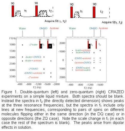
It turns out that both spins are flipped in the same direction (a “two-quantum transition”) for the peaks in the spectrum on the left. Both are flipped in opposite directions (a “zero-quantum transition”, because the net number of spins up does not change) for the spectrum on the right. In general a 1:n gradient pulse ratio produces peaks at the frequencies of “multiple-quantum coherences”, corresponding to a net flip of n spins; up to n=10 transitions have been observed. If n is not an integer, there is no signal (if only protons are excited); if protons and carbons are both excited (for example, coupling protons with hyperpolarized carbon nuclei ), peaks appear at the sum of the proton and carbon frequencies for a 4:5 gradient area ratio, and at the difference between the frequencies for a 4:3 gradient area ratio.
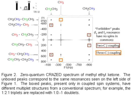
Note that there is nothing random about the patterns above. For example, in the zero-quantum spectrum, the water peak in the directly detected dimension is correlated with flipping two water spins (at zero frequency), one water and one DMSO spin, or one water and one acetone spin, but not with one DMSO and one acetone spin. In coupled spin systems, these other (“forbidden”) peaks can also appear, but again the structure is very strange. Figure 2 shows the zero-quantum spectrum of methyl ethyl ketone taken with the same sequence as on the right side of Figure 1. The three different types of protons (labeled in red, blue and green) generate the normally expected quartet, singlet and triplet in the directly detected dimension. In the other dimension, the same lines appear as in Figure 1, but additional zero-quantum transitions with quite different splittings also appear. For example, the methyl protons in the CH3CH2- group give a 1:0:-1 doublet, instead of a 1:2:1 triplet; the methylene protons give a 1:-1:-1:1 quartet instead of 1:3:3:1.
These spectra (and many more like them) were obtained several years ago. They raised several very fundamental questions (plus a tremendous amount of controversy). The standard picture of NMR made some assumptions that were defensible when solution NMR was first discovered (1948), but which became suspect as magnetic fields increased (by a factor of 30) and were never re-examined. We corrected the quantum mechanical framework, and discovered that these additional peaks come from transitions that require multiple spin flips, on molecules separated by many microns. We call these “intermolecular multiple-quantum coherences” or iMQCs. They are only observable because of the dipolar interaction between nuclei. Dipolar interactions themselves are not new in NMR: it has been known for half a century that liquids (such as water) give sharp NMR lines, and solids (such as ice) give NMR lines 10,000 times broader. This difference arises because the classical interaction energy E for a pair of magnetic dipoles µ in a large external magnetic field is E=µ2 (3cos2(θ)-1)/r3(r is the separation between the nuclei, θ is the angle between the internuclear vector and the applied magnetic field) and in a solid, each nucleus interacts with all other nuclei. In a liquid, Bloembergen pointed out in 1948 that diffusion averages the value of θ on an NMR time scale, and since <3cos2(θ)-1> the couplings are expected to disappear (Figure 3). Hence chemical shifts and J couplings, which are much smaller than dipolar couplings in solids, can be resolved in liquids– making NMR invaluable as a structural tool.
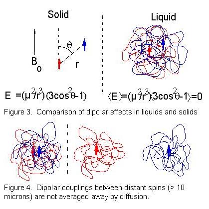
In fact, this seemingly simple and obvious argument is incorrect. Water molecules (diffusion constant D=2.3 x 10⁻⁹ m2•s-1) diffuse on average about 70µm along the internuclear vector in 1 second, the typical length of a free induction decay, so diffusion only averages away the coupling between spins separated by much less than this distance (Figure 4). This might seem quite sufficient, since the dipolar interaction falls as r-3; the dipolar coupling between two protons separated by 100µm would cause a 1 picoHertz line shift, only observable after 30,000 years of time evolution! However, the number of spins at a distance r is proportional to r2 dr. Thus the net magnetic field at any site from all the spins at a distance r only falls as 1/r, and the integral diverges–the spins between 1 and 3 mm from any given molecule are just as important as the ones between 1 and 3 Å! Experimentally liquids do give sharper lines than solids, but the real reason why dipolar couplings are not observed in liquids is much more subtle. If the sample is nearly spherical and the magnetization points in the same direction everywhere, the sum of all of the couplings vanishes. Breaking the spherical symmetry of the magnetization (for example, with an odd-shaped sample) reintroduces effects of the dipole-dipole coupling. At 30 MHz (the proton resonance frequency for the magnets used in the 1940s) we now know that the maximum residual effect from dipolar couplings is only about 0.1 Hz–far less than the linewidth available at the time. For concentrated samples in modern magnets, with nearly 30 times this field strength, the magnitude of the reintroduced dipolar coupling can be comparable to a J coupling (2-3 Hertz)–large enough to alter two-dimensional spectra and generate cross¬peaks, but not so large as to degrade resolution.
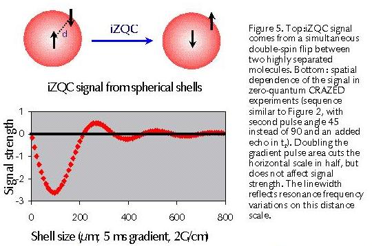
J couplings have been seen for decades: why wasn’t this effect observed? The reason is simple: in ordinary NMR tubes the active region in the probe is only about as long as it is wide, so the deviation from a sphere for the active region is small, and again the effect turns out to be small. However, gradient pulses can break the magnetization symmetry in a controlled way. During the gradient spins in different positions precess at different rates, so the magnetization gets wound up into a helix–for example, a 5 ms pulse with 2G/cm gradient strength gives a helix with a repeat distance of 230 µm. At half the repeat distance of the helix (which we call the correlation distance) the spherical symmetry is completely broken, and dipolar couplings are recovered. Figure 5 shows the calculated intermolecular zero-quantum coherence (iZQC) signal contributions from spherical shells of different sizes. Doubling the gradient pulse area cuts the correlation distance in half, but does not affect signal strength if the sample is homogeneous. However, the linewidth is dictated by the resonance frequency difference at the correlation distance, so CRAZED spectra can measure spatial correlations.